
CP2K
CP2K
CP2K is a quantum chemistry and solid state physics software package that can perform atomistic simulations of solid state, liquid, molecular, periodic, material, crystal, and biological systems. It provides the Quickstep (QS) module for density functional theory calculations using the Gaussian and plane waves (GPW) method, the FIST module for classical force field molecular dynamics, and modules for vibrational analysis, nudged elastic band transitions and TDDFPT excited states.
General Info
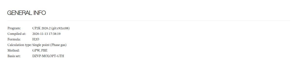
CP2K - General Info - Main fields
| Field | Description | Example |
|---|---|---|
| Program | CP2K program version used for the calculation | CP2K 2026.2 (git:c92cc08) |
| Compiled at | Build date of the CP2K binary | 2026-11-13 17:38:19 |
| Formula | Molecular formula in Hill notation, derived from the final geometry | H2O |
| Calculation type | Custom logic [^1] | Single point (Phase gas) |
| Method | QS method and exchange-correlation functional, joined as METHOD, FUNCTIONAL | GPW, PBE |
| Basis set | Basis sets of all atomic kinds, in the order they appear in the calculation. For hybrid functional calculations with ADMM, the auxiliary basis is not listed | DZVP-MOLOPT-GTH |
The calculation type may carry additional annotations: a , Electronic excitations suffix is added when TDDFPT excited states are computed, the phase in parentheses (Phase gas or the solvent name on solvated runs) tells the environment the energy refers to, and an ABORT marker flags runs that stopped on an error.
CP2K - General Info - HTML example
Atom Info
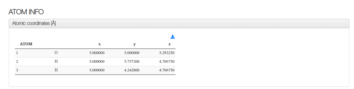
Displays the calculation geometry on an interactive JSmol viewer, along with a table of atomic coordinates in ångströms (Å). On periodic calculations the cell vectors are shown as well, and a download button allows exporting the geometry in XYZ format. When the upload includes the CP2K restart file of a geometry optimization, the initial and final geometries are displayed side by side.
Columns: atom index, element symbol, x, y, z (Å).
CP2K - Atom Info - HTML example
Molecular Info
Shows molecular-level properties of the system.
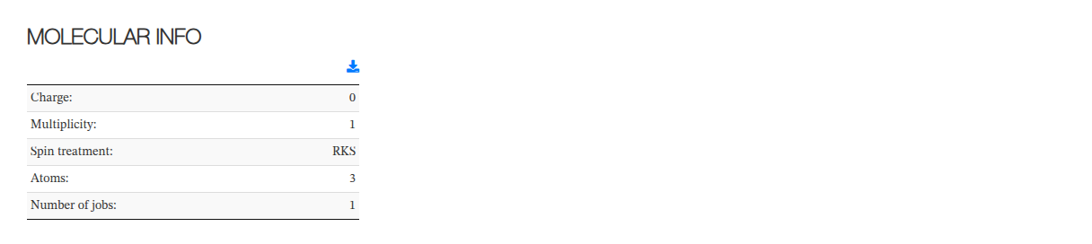
Molecular Info - Main fields
| Field | Description |
|---|---|
| Charge | Total net charge of the system, as defined on the input &FORCE_EVAL section |
| Multiplicity | Spin multiplicity of the system |
| Spin treatment | Restricted (RKS) or unrestricted (UKS) Kohn-Sham treatment |
| Atoms | Number of atoms in the system |
| Number of jobs | Number of runs found in the uploaded output; each job gets its own report section |
Molecular Info - HTML example
Modules
When a calculation contains multiple jobs, each is shown as a collapsible section with the subsections below (when applicable).
Parameters
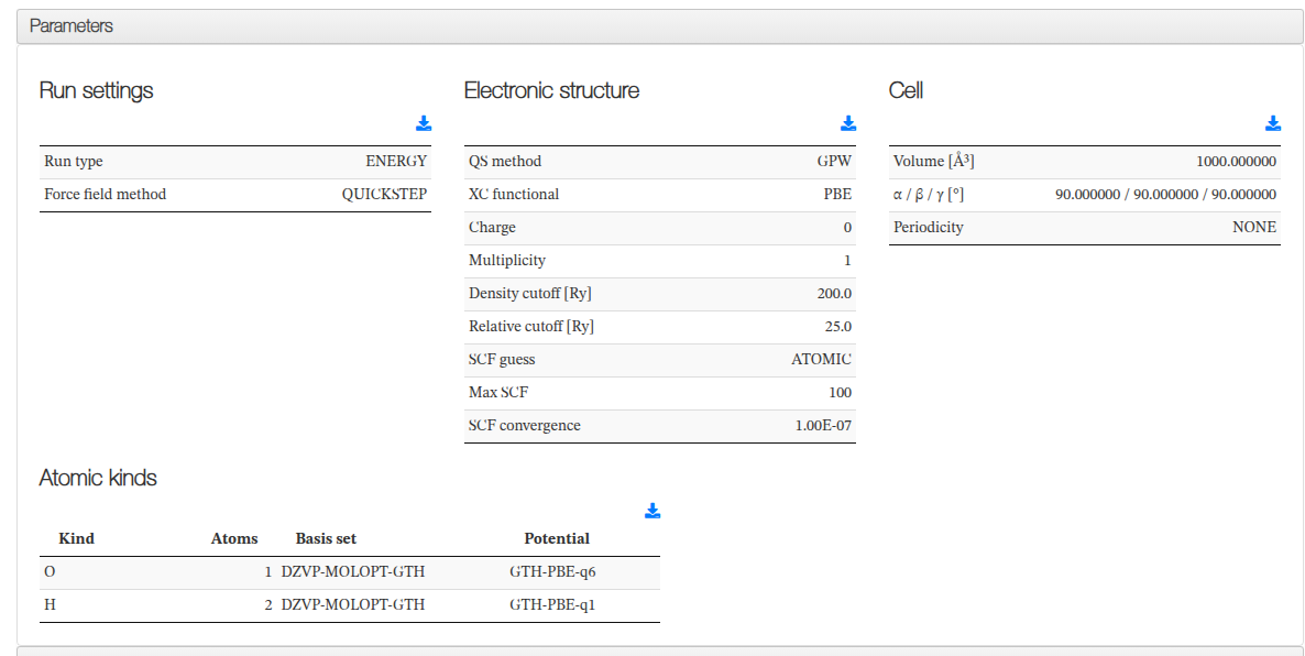
A collapsible panel lists the calculation setup parsed from the CP2K input and the run header, grouped into themed sub-tables: run settings, electronic structure, cell and, on molecular dynamics runs, the MD setup. A final table lists the atomic kinds with their basis set and pseudopotential.
Parameters - Displayed fields
| Group | Field | Description |
|---|---|---|
| Run settings | Run type | RUN_TYPE of the calculation (ENERGY, ENERGY_FORCE, GEO_OPT, CELL_OPT, MD, VIBRATIONAL_ANALYSIS, BAND) |
| Force field method | Quickstep (electronic structure) or FIST (classical force field) | |
| Dispersion | Dispersion correction, when defined (only shown when present) | |
| Thermostat | Thermostat used on molecular dynamics runs (only shown when present) | |
| Electronic structure | QS method | Gaussian and plane waves method (GPW) or related |
| XC functional | Exchange-correlation functional, including hybrid fractions on ADMM runs | |
| Charge / Multiplicity | Charge and spin multiplicity | |
| Density cutoff [Ry] | Plane wave density cutoff | |
| Relative cutoff [Ry] | Relative density cutoff for the mapping grid | |
| SCF guess | Initial guess for the SCF | |
| Max SCF | Maximum number of SCF iterations | |
| SCF convergence | Requested SCF convergence threshold on the energy | |
| Cell | Volume [ų] | Simulation cell volume |
| α / β / γ [°] | Cell angles | |
| Periodicity | Periodic directions (NONE, XY, XYZ) | |
| K-points in set | Number of k-points, only shown on k-point sampled calculations | |
| Molecular dynamics | Ensemble | MD ensemble (NVE, NVT, NPT_I, ...), only shown on MD runs |
| Steps | Number of MD steps | |
| Time step [fs] | Integration time step | |
| Temperature [K] | Reference temperature | |
| Atomic kinds | Kind | One row per atomic kind: element, number of atoms, basis set and pseudopotential (GTH-PBE-q6) |
Parameters - HTML example
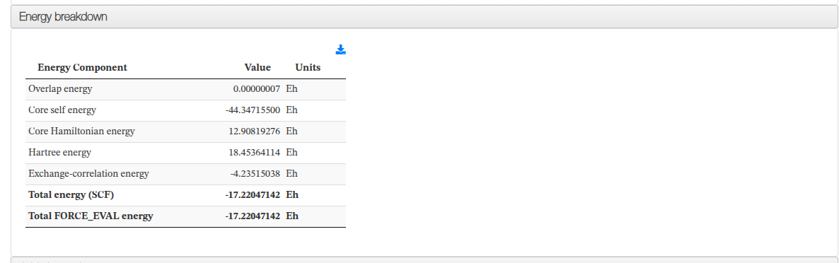
Energy Breakdown
Presents the energy contributions printed at the end of each SCF convergence, in Hartree (Eh). On vibrational analysis calculations the reference geometry energy replaces the SCF terms. Each row is shown only when the corresponding value is present, so dispersion-corrected runs add a dispersion energy row.
Energy Breakdown - Main fields
| Field | Description |
|---|---|
| Overlap energy | Core overlap energy (Eh) |
| Core self energy | Atomic core energies (Eh) |
| Core Hamiltonian energy | Kinetic and electron-nuclear contribution (Eh) |
| Hartree energy | Classical electrostatic electron-electron energy (Eh) |
| Exchange-correlation energy | XC contribution, including the exact exchange fraction on hybrid runs (Eh) |
| Dispersion energy | Dispersion correction, printed on DFT-D3 or similar runs only (Eh) |
| Total energy (SCF) | Total energy of the converged SCF (Eh) |
| Total FORCE_EVAL energy | Final energy reported by the FORCE_EVAL section (Eh) |
| Reference geometry energy | Energy of the reference geometry, shown on vibrational analysis calculations instead of the SCF terms (Eh) |
Energy Breakdown - HTML example
Optimization Steps
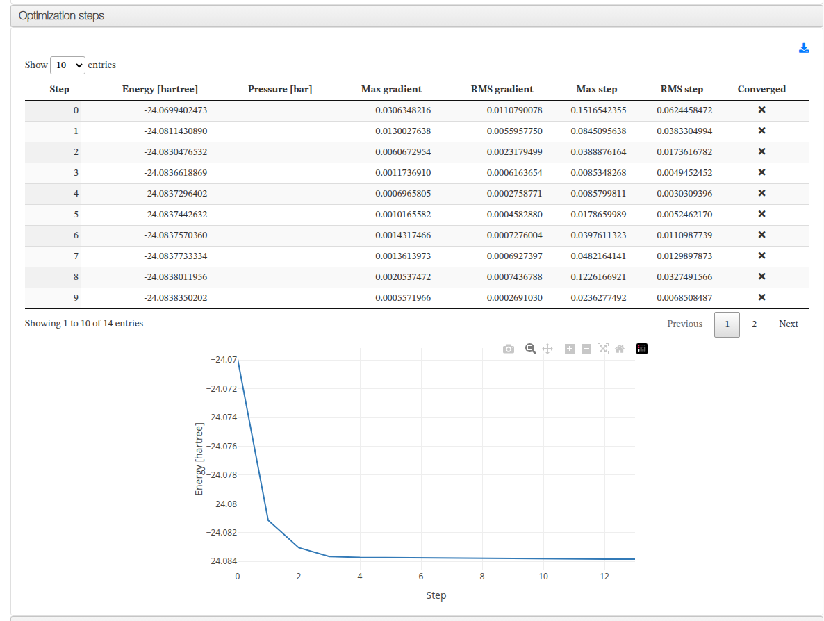
Shown on geometry and cell optimization runs. An interactive graph plots the energy, the convergence gradients and the step sizes along the optimization, and a data table lists every step.
Optimization Steps - Table columns
| Column | Description |
|---|---|
| Step | Optimization step number |
| Energy [hartree] | Total energy of the step |
| Pressure [bar] | Pressure of the step, printed on cell optimizations |
| Max gradient / RMS gradient | Maximum and root mean square gradient of the step |
| Max step / RMS step | Maximum and root mean square displacement of the step |
| Converged | Whether the step met the convergence criteria |
Optimization Steps - HTML example
Molecular Dynamics
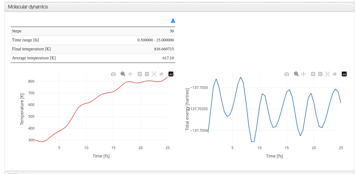
Shown on molecular dynamics runs. An interactive graph plots the temperature, kinetic and potential energy of every step, and the trajectory can be played on the JSmol viewer of the Atom Info section. A summary table describes the run.
Molecular Dynamics - Main fields
| Field | Description |
|---|---|
| Steps | Number of steps found in the output |
| Time range [fs] | First and last simulated time of the trajectory |
| Final / Average temperature [K] | Temperature of the last step and average along the run |
| Final pressure [bar] | Pressure of the last step, printed on NPT runs |
| Final volume [ų] | Cell volume of the last step, printed on variable cell runs |
Molecular Dynamics - HTML example
NEB Band Profile
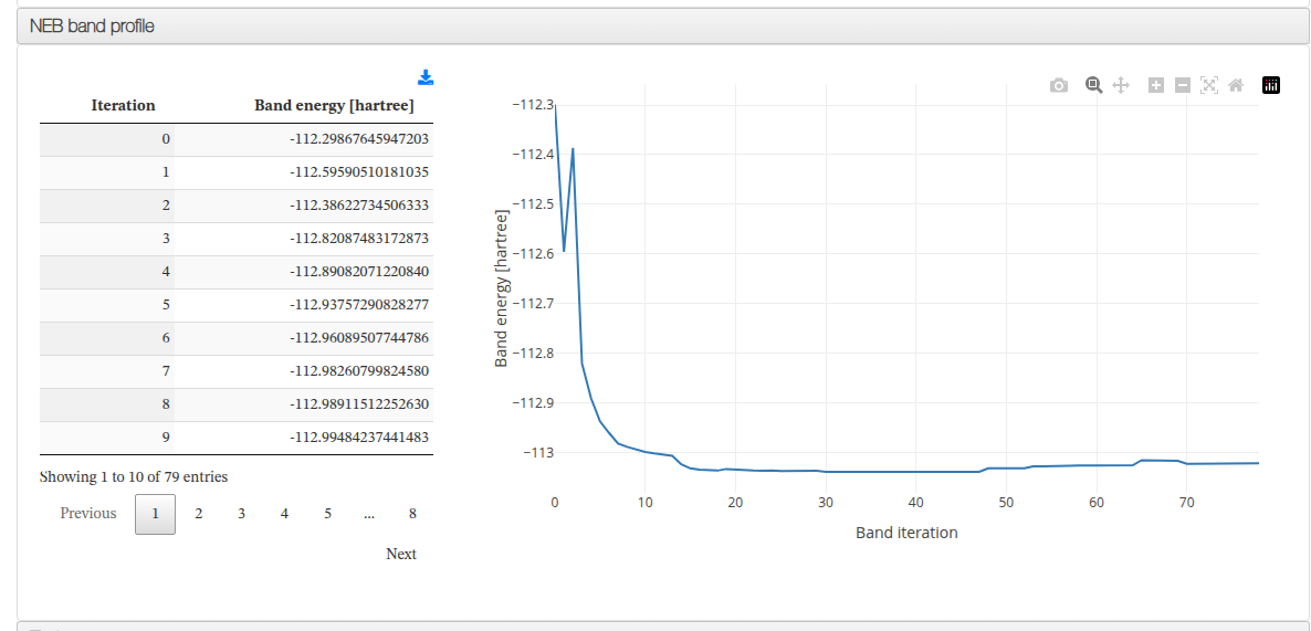
Shown on nudged elastic band (BAND run type) calculations. An interactive graph plots the band energy along the optimization and a data table lists the band energy of every iteration.
NEB Band Profile - Table columns
| Column | Description |
|---|---|
| Iteration | NEB optimization iteration number |
| Band energy [hartree] | Total energy of the band at that iteration |
NEB Band Profile - HTML example
Orbital Energies
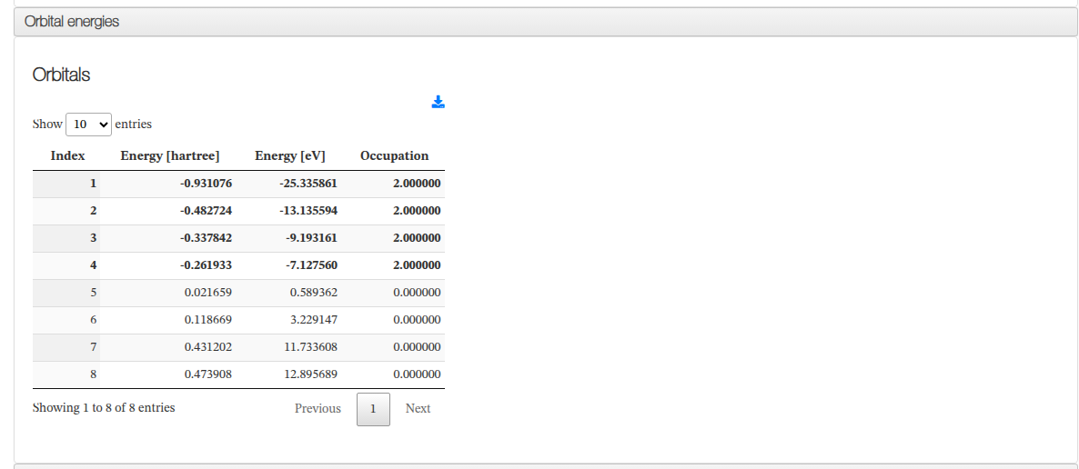
A collapsible panel lists the molecular orbital energies, when printed. For each orbital, the energy in Hartree and electronvolts and the occupation number are shown. Spin-unrestricted (UKS) calculations display two tables, one for the alpha and one for the beta orbitals. The table is sortable and paginated.
Orbital Energies - Table columns
| Column | Description |
|---|---|
| Index | Orbital index number |
| Energy [hartree] / Energy [eV] | Orbital energy in Hartree and electronvolts |
| Occupation | Electron occupation number of the orbital |
Orbital Energies - HTML example
Population Analysis
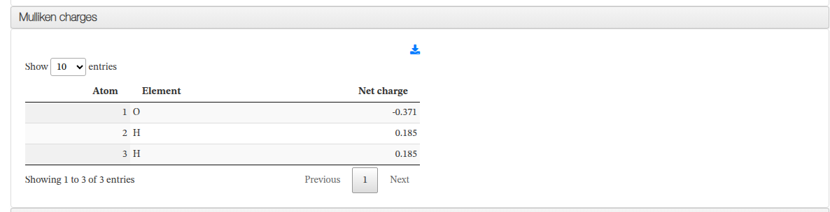
When printed, two collapsible panels present the Mulliken and the Hirshfeld charges of every atom. On spin-unrestricted (UKS) calculations each table adds a spin moment column with the difference between alpha and beta populations.
Mulliken / Hirshfeld charges - Table columns
| Column | Description |
|---|---|
| Atom | Atom index number |
| Element | Element symbol |
| Net charge | Atomic charge (e) |
| Spin moment | Alpha minus beta population of the atom, shown on UKS calculations (e) |
Mulliken charges - HTML example
Dipole Moment
When printed, a collapsible panel presents the electric dipole moment of the system.
Dipole Moment - Main fields
| Field | Description |
|---|---|
| x [D], y [D], z [D] | Cartesian components of the dipole moment (Debye) |
| Total [D] | Dipole moment magnitude (Debye) |
Dipole Moment - HTML example

IR Spectrum
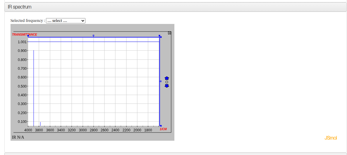
Shown on vibrational analysis calculations. Displays the infrared spectrum computed from the analytic frequencies and intensities using the JCAMP-DX plugin, alongside a molecular viewer synchronized to the selected vibrational mode. A dropdown allows selecting individual frequencies.
IR Spectrum - HTML example
Electronic Excitations (TDDFPT)
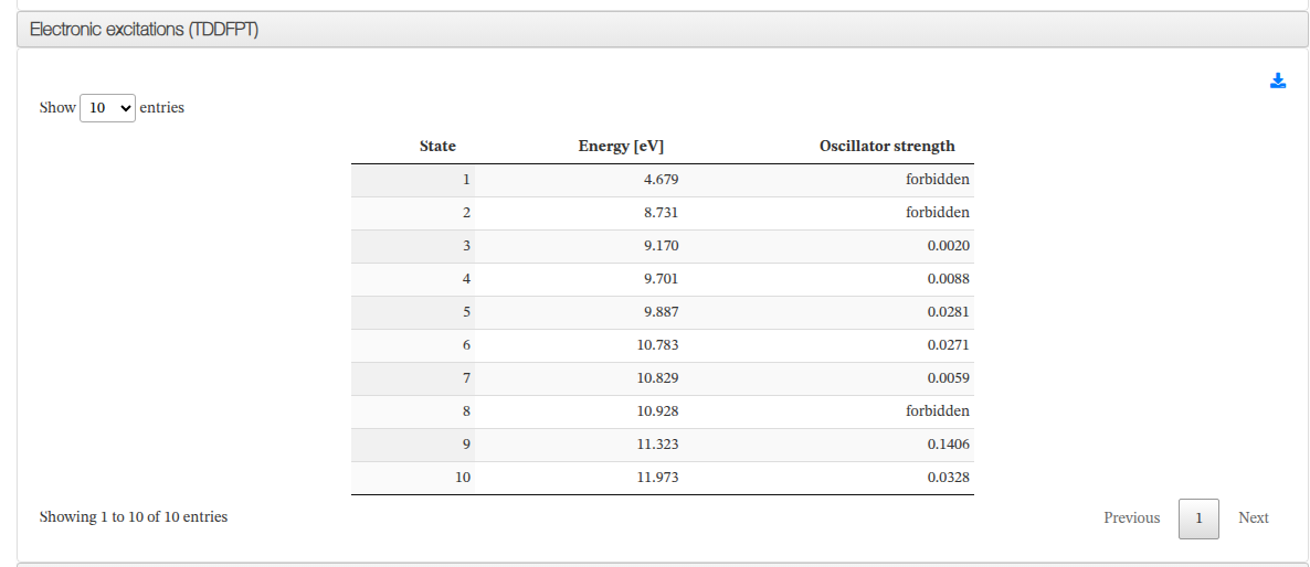
Shown on calculations that compute excited states by time-dependent density functional perturbation theory. A collapsible panel lists every excitation; dipole-forbidden states are labeled as such instead of showing a numeric oscillator strength.
Electronic Excitations - Table columns
| Column | Description |
|---|---|
| State | Excited state number |
| Energy [eV] | Excitation energy of the state |
| Oscillator strength | Oscillator strength of the transition, or the forbidden label for dipole-forbidden states |
Electronic Excitations - HTML example
Solvation Input
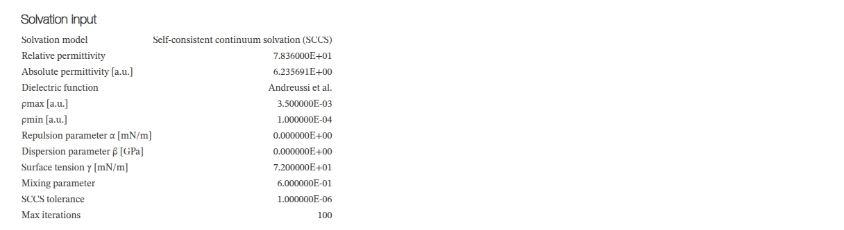
Shown on calculations that use the self-consistent continuum solvation (SCCS) model. A table placed before the job sections collects the solvation parameters as defined on the input, and the reported energy refers to the solvated system.
Solvation Input - Main fields
| Field | Description |
|---|---|
| Solvation model | Implicit solvation model name |
| Relative permittivity | Relative permittivity of the solvent |
| Absolute permittivity [a.u.] | Absolute permittivity in atomic units |
| Dielectric function | Dielectric function used by the model |
| ρmax [a.u.] / ρmin [a.u.] | Density thresholds of the solute cavity |
| Repulsion parameter α [mN/m] | Repulsion contribution of the cavitation free energy |
| Dispersion parameter β [GPa] | Dispersion contribution of the cavitation free energy |
| Surface tension γ [mN/m] | Surface tension of the solvent |
| Mixing parameter | Fraction of the potential used in the self-consistent iteration |
| SCCS tolerance | Convergence threshold of the continuum |
| Max iterations | Maximum number of continuum iterations |
Solvation Input - HTML example
Timings
Reports the elapsed CPU time and the completion timestamp of the calculation.
Timings - Main fields
| Field | Description |
|---|---|
| Elapsed CPU time [s] | Total CPU time reported at the end of the run |
| Finished at | Date and time when the calculation finished |
Timings - HTML example

[^1]: string cp2k:getCalcType node() job
        <xsl:variable name="runType" as="xs:string?"
            select="string(($job//parameter[@dictRef='cp2k:runType']/scalar)[1])"/>
        <xsl:variable name="status" as="xs:string?"
            select="string(($job//property[@dictRef='cp2k:status']/scalar |
                            $job//scalar[@dictRef='cp2k:status'])[1])"/>
        <xsl:variable name="notConverged" select="$status = 'not converged'"/>

        <xsl:choose>
            <xsl:when test="$runType = 'GEO_OPT'">
                <xsl:sequence select="if($notConverged) then $cp2k:GeometryOptimizationNotConverged
                                      else $cp2k:GeometryOptimization"/>
            </xsl:when>
            <xsl:when test="$runType = 'CELL_OPT'">
                <xsl:sequence select="if($notConverged) then $cp2k:CellOptimizationNotConverged
                                      else $cp2k:CellOptimization"/>
            </xsl:when>
            <xsl:when test="$runType = 'MD'">
                <xsl:sequence select="$cp2k:MolecularDynamics"/>
            </xsl:when>
            <xsl:when test="$runType = 'VIBRATIONAL_ANALYSIS'">
                <xsl:sequence select="$cp2k:FrequencyCalculation"/>
            </xsl:when>
            <xsl:when test="$runType = 'BAND'">
                <xsl:sequence select="$cp2k:NudgedElasticBand"/>
            </xsl:when>
            <xsl:when test="$runType = 'ENERGY_FORCE'">
                <xsl:sequence select="$cp2k:SinglePointForces"/>
            </xsl:when>
            <xsl:otherwise>
                <xsl:sequence select="$cp2k:SinglePoint"/>
            </xsl:otherwise>
        </xsl:choose>

        <!-- TDDFPT excitations can accompany any ground-state run type -->
        <xsl:if test="exists($job//property[@dictRef='cp2k:excitationEnergy'] |
                            $job//array[@dictRef='cp2k:excitationEnergy'])">
            <xsl:sequence select="$cp2k:ElectronicTransitions"/>
        </xsl:if>