
xTB
xTB
xTB (extended tight-binding) is a semiempirical quantum chemistry program based on density functional tight-binding (DFTB) methods. It provides fast geometry optimizations, molecular dynamics, and property predictions for molecular systems using GFN-xTB models.
General Info
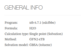
XTB - General Info - Main fields
| Field | Description | Example |
|---|---|---|
| Title | Calculation title, assigned during publication | Sample calculation |
| Browse Item | Link to the published item in the Browse repository | https://iochem-bd.iciq.es/browse/handle/100/5672 |
| Program | XTB program version used for the calculation | xtb 6.5.1 (git b0914e9) |
| Author | Full name of the user who submitted the calculation | Doe, John |
| Formula | Molecular formula in Hill notation, derived from the final geometry | C 6 H 6 |
| Calculation type | Custom logic [^1] | Geometry optimization |
| Method | GFN-xTB model variant used for the calculation. Runs driven by tblite do not name the Hamiltonian in the log, so for those the variant is derived from the GFN version requested on the command line | GFN2-xTB |
| Solvation model | Implicit solvation model followed by the solvent, in the form MODEL (solvent). The solvent is taken from the command line when it is named there: a CPCM-X run therefore reports the requested solvent instead of the ideal-conductor reference its SCF stage runs against (only shown when solvation is enabled) | ALPB (water) |
| Optimization | Convergence status of the geometry optimization (only shown for optimization runs) | Converged |
XTB - General Info - HTML example
Calculation Setup
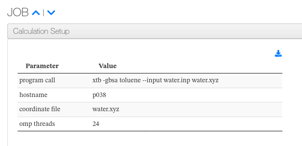
For each job, a collapsible panel lists the calculation setup parameters parsed from the XTB run header. Each row displays the parameter name alongside its configured value.
Calculation Setup - Displayed fields
| Column | Description |
|---|---|
| Parameter | Name of the setup parameter (e.g. program call, method, charge) |
| Value | Configured value for the parameter |
Calculation Setup - HTML example
Atom Info
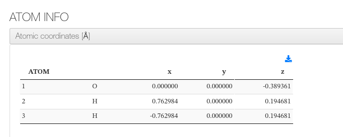
Displays a table of atomic coordinates in ångströms (Å). The final geometry is shown when available; otherwise the initial structure is displayed. A download button allows exporting the geometry in XYZ format.
Columns: atom index, element symbol, x, y, z (Å).
XTB - Atom Info - HTML example
Bond Distances
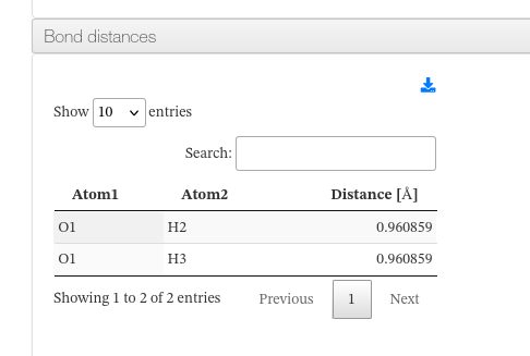
When bond information is available, a collapsible panel displays the pairwise bond distances computed from the Cartesian coordinates. Each row identifies the two bonded atoms (element symbol + serial number) and the distance in ångströms (Å).
Bond distances - HTML example
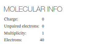
Molecular Info
Shows molecular-level electronic properties of the system.
Molecular Info - Main fields
| Field | Description |
|---|---|
| Charge | Total net electrical charge of the system. Read from the log when it reports one, otherwise from the input file, otherwise the xTB default of 0 |
| Unpaired electrons | Number of unpaired electrons, that is Nalpha - Nbeta. Read from the log when it reports one, otherwise from the input file, otherwise the xTB default: 0 for an even electron count and 1 for an odd one |
| Multiplicity | Spin multiplicity, computed as unpaired electrons + 1 (only shown when the number of unpaired electrons is known) |
| Electrons | Valence electron count reported by the tblite driver. It is what determines the default number of unpaired electrons (only shown when present) |
Molecular Info - HTML example
Modules
When a calculation contains multiple jobs, each is shown as a collapsible section with the subsections below (when applicable).
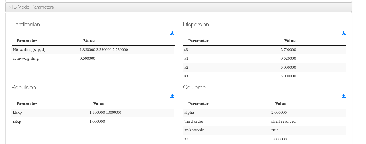
xTB Model Parameters
A collapsible panel displays the xTB model parameters grouped by section (Hamiltonian, Dispersion, Repulsion, Coulomb, Solvation, etc.). Each group is rendered as a separate sub-table with two columns: parameter name and value.
xTB Model Parameters - Common groups
| Group | Description |
|---|---|
| Hamiltonian | Method and Hamiltonian settings (e.g. GFN2-xTB) |
| Dispersion | Dispersion correction parameters |
| Repulsion | Repulsive potential parameters |
| Coulomb | Coulomb interaction parameters |
| Solvation | Implicit solvation model parameters (when solvation is enabled) |
xTB Model Parameters - HTML example
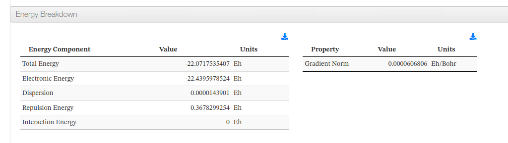
Energy Breakdown
Presents the total energy and its individual contributions from the final summary of the calculation. A second table shows the gradient norm, HOMO-LUMO gap and Fermi level. All energy values are displayed in Hartree (Eh).
Not every run prints every contribution, and each row is shown only when the corresponding value is present. Solvated runs add the Gsolv decomposition and the total energy without the Gsasa and Ghb terms. Runs driven by tblite print no summary table at all: for those the values come from the final totals box and from the energy terms tblite reports around the SCF, which is where Electronic Energy and Interaction Energy originate.
Energy Breakdown - Main fields
| Field | Description |
|---|---|
| Total Energy | Total electronic energy of the system (Eh) |
| Total w/o Gsasa/Ghb | Total energy excluding the surface-area and hydrogen-bond solvation terms, printed by solvated runs only (Eh) |
| SCC Energy | Self-consistent charge contribution (Eh) |
| Electronic Energy | Electronic contribution reported by the tblite driver (Eh) |
| Isotropic ES | Isotropic electrostatic energy (Eh) |
| Anisotropic ES | Anisotropic electrostatic energy (Eh) |
| Anisotropic XC | Anisotropic exchange-correlation energy (Eh) |
| Dispersion | Dispersion correction energy (Eh) |
| Gsolv | Total free energy of solvation, printed by solvated runs only (Eh) |
| -> Gelec | Electrostatic part of the solvation free energy (Eh) |
| -> Gsasa | Surface-area (cavity and dispersion) part of the solvation free energy (Eh) |
| -> Ghb | Hydrogen-bonding part of the solvation free energy (Eh) |
| -> Gshift | Reference-state shift applied to the solvation free energy (Eh) |
| Repulsion Energy | Repulsive pair-potential energy (Eh) |
| Interaction Energy | Interaction energy reported by the tblite driver (Eh) |
| Additional Restraining | Restraint energy contribution (Eh) |
| Gradient Norm | Maximum gradient norm, indicating convergence quality (Eh/bohr) |
| HOMO-LUMO Gap | Energy gap between the highest occupied and lowest unoccupied molecular orbitals (eV) |
| Fermi Level | Fermi level of the system, printed under the orbital table (Eh) |
Energy Breakdown - HTML example
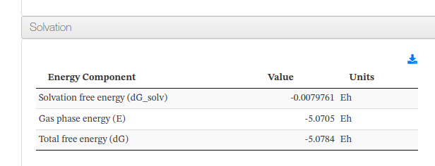
Solvation
Shown for runs that perform a CPCM-X post-SCF solvation evaluation. The SCF itself is solved against the ideal conductor, so this panel holds the only energies in such a log that refer to the solvent actually requested. All values are displayed in Hartree (Eh).
Solvation - Main fields
| Field | Description |
|---|---|
| Solvation free energy (dG_solv) | Free energy of transferring the solute from the gas phase into the solvent (Eh) |
| Gas phase energy (E) | Energy of the solute in the gas phase (Eh) |
| Total free energy (dG) | Gas phase energy plus the solvation free energy (Eh) |
Solvation - HTML example
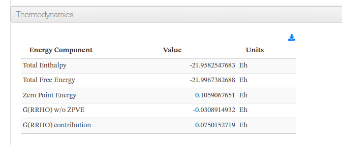
Thermodynamics
Shown for runs that compute a Hessian, which are the only ones that print thermochemical data. The values are taken from the thermodynamic summary and from the final totals box. Each row is shown only when the corresponding value is present, so a run that reports part of the table still renders. All values are displayed in Hartree (Eh).
Thermodynamics - Main fields
| Field | Description |
|---|---|
| Total Enthalpy | Total enthalpy of the system at the reported temperature (Eh) |
| Total Free Energy | Total Gibbs free energy of the system (Eh) |
| Zero Point Energy | Vibrational zero point energy (Eh) |
| G(RRHO) w/o ZPVE | Thermal free energy contribution from the rigid rotor harmonic oscillator treatment, excluding the zero point vibrational energy (Eh) |
| G(RRHO) contribution | Total rigid rotor harmonic oscillator contribution to the free energy, zero point vibrational energy included (Eh) |
Thermodynamics - HTML example
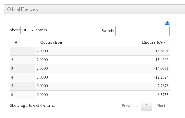
Orbital Energies
A collapsible panel lists the molecular orbital energies. For each orbital, the occupation number and energy are shown. The table is sortable and paginated.
Orbital Energies - Table columns
| Column | Description |
|---|---|
| # | Orbital index number |
| Occupation | Electron occupation number of the orbital |
| Energy | Orbital energy in electronvolts (eV) |
Orbital Energies - HTML example
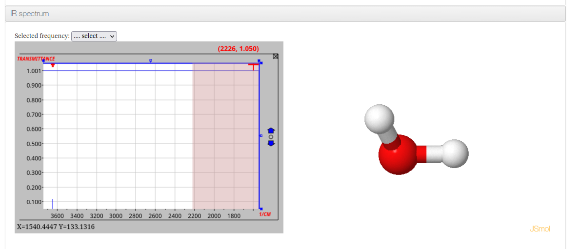
IR Spectrum
Shown when vibrational frequency data is available. Displays an interactive IR spectrum alongside a molecular viewer synchronized to the selected vibrational mode. A dropdown allows selecting individual frequencies.
IR Spectrum - HTML example
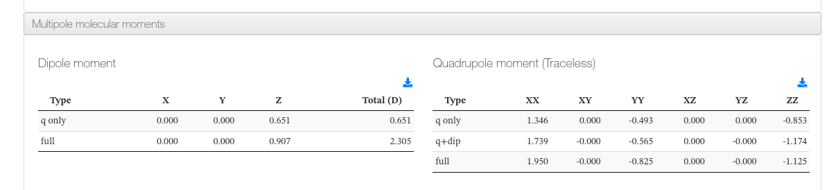
Multipole Moments
When available, a collapsible panel presents the dipole and quadrupole moments of the molecule.
Dipole Moment - Main fields
| Field | Description |
|---|---|
| q only (X, Y, Z) | Charge-only contribution to the dipole moment along each axis (Debye) |
| q only total (D) | Total charge-only dipole magnitude (Debye) |
| full (X, Y, Z) | Full dipole moment (charge + orbital contributions) along each axis (Debye) |
| full total (D) | Total dipole moment magnitude including all contributions (Debye) |
Quadrupole Moment (traceless) - Main fields
| Field | Description |
|---|---|
| q only | Charge-only contribution to the traceless quadrupole tensor (XX, XY, YY, XZ, YZ, ZZ) |
| q+dip | Charge + dipole contribution to the traceless quadrupole tensor |
| full | Full quadrupole tensor including all contributions |
Multipole Moments - HTML example
Timing
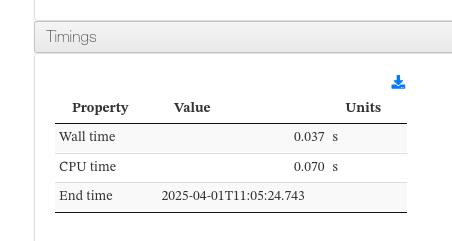
Reports the wall-clock time, CPU time, and completion timestamp of the calculation.
Timing - Main fields
| Field | Description |
|---|---|
| Wall time | Total elapsed wall-clock time for the calculation |
| CPU time | Total CPU time consumed across all cores |
| End time | Date and time when the calculation finished |
Timing - HTML example
[^1]: string xtb:getCalcType boolean hasOptimization boolean isConverged
        <xsl:variable name="xtb:SinglePoint" select="'Single point'" />
        <xsl:variable name="xtb:GeometryOptimization" select="'Geometry optimization'" />
        <xsl:variable name="xtb:GeometryOptimizationNotConverged" select="'Geometry optimization (not converged)'" />
        <xsl:variable name="xtb:FrequencyCalculation" select="'Frequency calculation'" />
        <xsl:variable name="xtb:SinglePointHessian" select="'Single point Hessian (SPH)'" />
        <xsl:variable name="xtb:MolecularDynamics" select="'Molecular dynamics'" />
        <xsl:variable name="xtb:MetaDynamics" select="'Meta-dynamics'" />


         <xsl:function name="xtb:getCalcType" as="xs:string*">
            <xsl:param name="cml" as="node()"/>

            <!-- Get program call from calculation.setup module -->
            <xsl:variable name="programCall" as="xs:string?"
                select="$cml//cml:module[@cmlx:templateRef='calculation.setup']
                        //cml:list[./cml:scalar[@dictRef='xtb:name']='program call']
                        /cml:scalar[@dictRef='xtb:value']"/>

            <xsl:choose>
                <!-- Check for metadynamics flag (\-\-metad) -->
                <xsl:when test="contains($programCall, '--metad')">
                    <xsl:sequence select="$xtb:MetaDynamics"/>
                </xsl:when>

                <!-- \-\-omd: geometry optimization + molecular dynamics -->
                <xsl:when test="contains($programCall, '--omd')">
                    <xsl:sequence select="xtb:getOptimizationStatus($cml)"/>
                    <xsl:sequence select="$xtb:MolecularDynamics"/>
                </xsl:when>

                <!-- \-\-md: molecular dynamics only -->
                <xsl:when test="contains($programCall, '--md')">
                    <xsl:sequence select="$xtb:MolecularDynamics"/>
                </xsl:when>

                <!-- \-\-ohess: geometry optimization + frequency calculation -->
                <xsl:when test="contains($programCall, '--ohess')">
                    <xsl:sequence select="xtb:getOptimizationStatus($cml)"/>
                    <xsl:sequence select="$xtb:FrequencyCalculation"/>
                </xsl:when>

                <!-- \-\-hess or \-\-freq: frequency calculation only -->
                <xsl:when test="contains($programCall, '--hess') or contains($programCall, '--freq')">
                    <xsl:sequence select="$xtb:FrequencyCalculation"/>
                </xsl:when>

                <!-- \-\-opt: geometry optimization only, or fallback via ANCOPT section -->
                <xsl:when test="contains($programCall, '--opt') or
                                exists($cml//cml:module[@cmlx:templateRef='optimization'])">
                    <xsl:sequence select="xtb:getOptimizationStatus($cml)"/>
                </xsl:when>

                <!-- Default: Single Point calculation -->
                <xsl:otherwise>
                    <xsl:sequence select="$xtb:SinglePoint"/>
                </xsl:otherwise>
            </xsl:choose>
        </xsl:function>

        <!--
            Helper function to get optimization status.
            Returns the appropriate calculation type string based on convergence.
        -->
        <xsl:function name="xtb:getOptimizationStatus" as="xs:string">
            <xsl:param name="cml" as="node()"/>

            <xsl:variable name="convergedValue" as="xs:string?"
                select="$cml//cml:scalar[@dictRef='xtb:converged']"/>

            <xsl:choose>
                <!-- Converged optimization -->
                <xsl:when test="$convergedValue = 'converged'">
                    <xsl:sequence select="$xtb:GeometryOptimization"/>
                </xsl:when>

                <!-- Not converged optimization -->
                <xsl:when test="$convergedValue = 'notconverged'">
                    <xsl:sequence select="$xtb:GeometryOptimizationNotConverged"/>
                </xsl:when>

                <!-- ANCOPT present but convergence scalar missing - assume converged -->
                <xsl:when test="exists($cml//cml:module[@cmlx:templateRef='optimization'])">
                    <xsl:sequence select="$xtb:GeometryOptimization"/>
                </xsl:when>

                <!-- Fallback to single point -->
                <xsl:otherwise>
                    <xsl:sequence select="$xtb:SinglePoint"/>
                </xsl:otherwise>
            </xsl:choose>
        </xsl:function>